Job-Market Trend Analysis: A 5-Step Framework You Can Run in Python

Job market analytics is essential for making smart hiring decisions, along with planning your workforce strategy. When you are analyzing job data trends, you find valuable insights about salary changes, skill demands, industry growth patterns, and much more. Trend analysis is the backbone of the process of job market research. It helps you find patterns within employment data for any time period. You can spot roles with growth, skills employers want most, and movement of compensation packages. Trend analysis works by examining historical job posting data to forecast what’s coming next. This approach helps you stay ahead of industry changes and make decisions based on solid data rather than guesswork.

Job market analytics is built on the following components: 

• Time-series analysis tracks employment patterns across different periods 
• Seasonality detection identifies recurring hiring cycles throughout the year 
• Forecasting models predicts future job market conditions 
• Data smoothing techniques removes noise from raw employment statistics

You’ll pull labor market data from job boards, company career pages, and government databases. When you process this through specialized APIs, you get real-time market insights that actually matter for your planning. When you understand how trend analysis works, your strategic decisions get better.You’ll spot talent shortages early, know when to adjust compensation, and discover emerging job categories while your competitors are still catching up. 

The future of data science careers shows how trend analysis applies to specific industries. Market research reveals which technical skills will be most valuable in coming years. Companies using labor market analytics report better hiring outcomes and reduced time-to-fill positions. Trend analysis methods provide the foundation for these improved results.

Step 1: Connect to JobsPikr and Pull Raw Postings

Getting reliable job market data doesn’t have to be a nightmare. You can skip the headaches of building scrapers or cleaning messy datasets.

The JobsPikr job data API gives you structured access to millions of job postings worldwide. You get clean, standardized data that’s perfect for market trend analysis strategies and job market analytics.

Copy/Paste Environment Setup

export JOBSPIKR_API_KEY=”your_api_key_here”

export JOBSPIKR_BASE_URL=”https://api.jobspikr.com/v2″

Quick cURL Test

curl -X GET “https://api.jobspikr.com/v2/jobs?q=data+analyst&location=US&page_size=10” \

  -H “Authorization: Bearer $JOBSPIKR_API_KEY”

Python Implementation with Pandas

Here’s your production-ready data pull script:

import requests

import pandas as pd

from datetime import datetime, timedelta

import time

class JobDataPuller:

    def __init__(self, api_key):

        self.api_key = api_key

        self.base_url = “https://api.jobspikr.com/v2”

        self.headers = {“Authorization”: f”Bearer {api_key}”}

    def fetch_jobs(self, filters=None, max_pages=10):

        all_jobs = []

        page = 1

        default_filters = {

            ‘posted_after’: (datetime.now() – timedelta(days=7)).isoformat(),

            ‘page_size’: 100,

            ’employment_type’: ‘full-time’

        }

        params = {**default_filters, **(filters or {})}

        while page <= max_pages:

            params[‘page’] = page

            try:

                response = requests.get(

                    f”{self.base_url}/jobs”, 

                    headers=self.headers, 

                    params=params,

                    timeout=30

                )

                response.raise_for_status()

                data = response.json()

                jobs = data.get(‘jobs’, [])

                if not jobs:

                    break

                all_jobs.extend(jobs)

                page += 1

                time.sleep(0.5)  # Rate limiting

            except requests.exceptions.RequestException as e:

                print(f”Request failed: {e}”)

                break

        return all_jobs

Data Hygiene Checklist

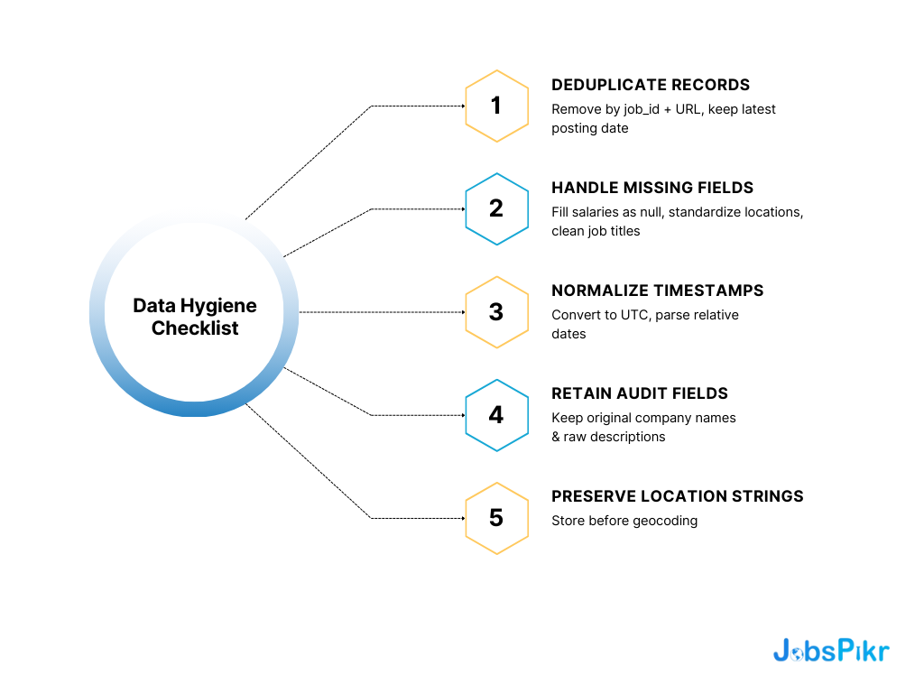
Your raw data needs cleaning before analysis. 

Here’s what to watch for:

Deduplicate Records

• Remove duplicates by job_id and URL combination
• Keep the most recent posting date

Handle Missing Fields

• Fill missing salaries with null values
• Standardize location formats
• Clean job titles of special characters

Normalize Timestamps

• Convert all posted_at fields to UTC
• Parse relative dates like “3 days ago”

Retain Audit Fields

• Keep original company names
• Store raw descriptions for keyword analysis
• Preserve location strings before geocoding

Expected Dataset Shape

After processing, your dataframe should look like this:

Column	Type	Example
job_id	string	“jp_12345”
title	string	“Senior Data Analyst”
company	string	“TechCorp Inc”
location	string	“San Francisco, CA”
posted_at	datetime	2025-09-10 14:30:00
salary_min	float	95000.0
employment_type	string	“full-time”
remote_allowed	boolean	True

Expect around 1,000-5,000 jobs per day for broad searches. Narrow filters yield 100-500 records.

Why API Beats DIY Scraping

Building your own scrapers seems tempting. But you’ll hit walls fast.

JobsPikr handles the messy stuff:

• Global coverage across 70K+ sources
• AI-driven processing removes expired postings
• Near real-time updates every few hours
• Structured JSON instead of raw HTML

DIY scraping means constant maintenance. Job boards change layouts weekly. Anti-bot measures block your requests. You spend more time fixing scrapers than analyzing trends.

Common Errors and Quick Fixes

401 Authentication Error

# Check your API key format

headers = {“Authorization”: “Bearer YOUR_KEY_HERE”}  # Not “Token” or “API-Key”

Rate Limit (429)

# Add delays between requests

time.sleep(1.0)  # Wait 1 second between calls

Empty Results

# Verify your filters aren’t too restrictive

params = {

    ‘q’: ‘analyst’,  # Broader search terms

    ‘location’: ‘US’,  # Country codes work better

    ‘posted_after’: (datetime.now() – timedelta(days=30)).isoformat()

}

Building Your First Dataset

Start with a focused pull to test your setup:

puller = JobDataPuller(“your_api_key”)

# Pull data analyst jobs from last week

filters = {

    ‘q’: ‘data analyst’,

    ‘location’: ‘US’,

    ‘posted_after’: ‘2025-09-04T00:00:00Z’

}

jobs = puller.fetch_jobs(filters, max_pages=5)

df = pd.DataFrame(jobs)

# Quick data check

print(f”Pulled {len(df)} jobs”)

print(df.head())

Triangulating this data with other sources like BLS employment statistics or LinkedIn workforce reports can be made part of your processes. But JobsPikr serves as your primary feed for fresh, structured labor market data.

Step 2: Normalize Job Titles, Skills, and Locations

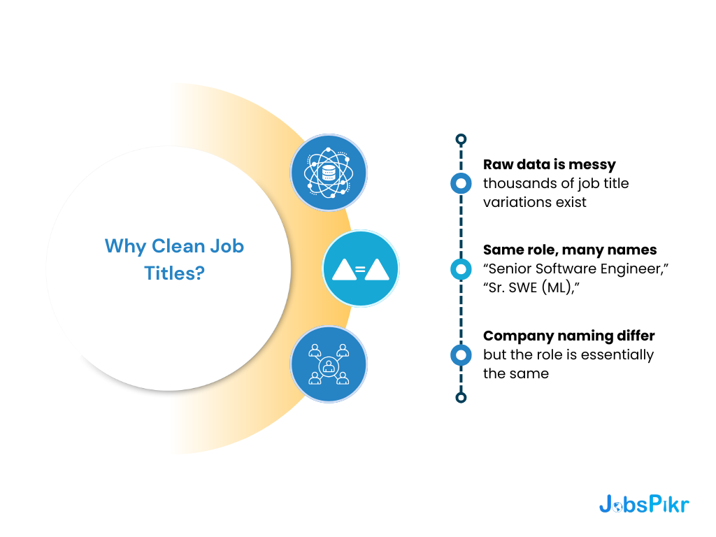
Before you can analyze trends in job market data, you need to clean up the chaos. Raw job postings contain thousands of title variations that represent the same roles. Your database might show “Senior Software Engineer,” “Sr. SWE (ML),” and “Software Engineer III” as three different roles. In reality, they’re the same position with different company naming styles.

The Scale of the Problem

Raw Title	Normalized Title
Sr. SWE (ML)	Software Engineer
Lead Dev – Frontend	Software Engineer
Accountant II	Accountant
Marketing Specialist III	Marketing Specialist

Most organizations see 15,000+ unique job titles that collapse into fewer than 1,000 actual roles after normalization.

Job Title Normalization Strategy

Start with a rules-first approach for common variations. Create lookup tables that handle frequent abbreviations and seniority levels.

import re

from sklearn.metrics.pairwise import cosine_similarity

# Stage 1: Rules-based mapping

title_mappings = {

    r’Sr\.?\s+’: ‘Senior ‘,

    r’\s+I{1,3}$’: ”,  # Remove Roman numerals

    r’Lead\s+’: ‘Senior ‘,

}

def normalize_title_rules(title):

    for pattern, replacement in title_mappings.items():

        title = re.sub(pattern, replacement, title)

    return title.strip()

For complex cases that rules miss, use semantic embeddings. Normalizing textual data with Python involves comparing title similarities using sentence transformers. The hybrid approach catches 90% of variations through simple rules. Machine learning handles the remaining edge cases.

Taxonomy Alignment

Consider mapping your normalized titles to standard frameworks like ONET-SOC. This 900+ occupation classification system enables external benchmarking and regulatory compliance. You can also build custom taxonomies for industry-specific roles. Many companies use hybrid approaches that layer internal categories over ONET foundations.

Skills Extraction and Normalization

Skills data suffers from similar inconsistencies. “PostgreSQL,” “Postgres,” and “psql” all refer to the same database technology. Use named entity recognition to extract skills from job descriptions. Then apply synonym resolution to group related terms.

import spacy

# Extract skills using NER

nlp = spacy.load(“en_core_web_sm”)

def extract_skills(text):

    doc = nlp(text)

    skills = []

    for ent in doc.ents:

        if ent.label_ in [“TECH”, “SKILL”]:

            skills.append(ent.text)

    return skills

Create skill families that group individual technologies. Map “React,” “Node.js,” and “JavaScript” under “Frontend Development” for trend analysis.

Location Standardization

Geographic data presents unique challenges for job market analytics. You’ll encounter “NYC,” “New York, NY,” and “Remote – United States” in the same dataset. Implement geocoding to resolve locations to consistent formats:

• Latitude/longitude coordinates
• Canonical place names
• Administrative hierarchies (City → State → Country)
• ISO country codes
• Time zone information

Time zones help create meaningful weekly trend buckets. Remote work positions need special handling with governing jurisdictions for legal compliance.

Quality Control Loop

• Build active learning workflows to improve normalization accuracy. Flag low-confidence mappings for human review.
• Track key metrics like coverage rates and precision scores. Monitor how many raw titles successfully map to canonical forms versus requiring manual intervention.
• Update your normalization rules based on reviewer feedback. This creates a continuous improvement cycle that adapts to new job titles and industry terminology.

Privacy and Compliance

• Make sure your normalization process keeps personally identifiable information locked down. Strip company-specific prefixes and candidate names from title strings.
• Store normalized data separately from raw inputs to maintain audit trails. This helps with compliance reviews and debugging normalization issues.
• The normalized data becomes your foundation for meaningful trend analysis. Clean categories enable accurate aggregations and more stable forecasting models.

Step 3: Transform to Weekly Time Series and Chart Hiring Velocity

Once you have your cleaned job posting data, the next step involves aggregating daily events into weekly buckets. This transformation makes patterns clearer and reduces noise in your analysis.

Converting to Weekly Aggregates

Start by working with time series data in Python through pandas. You’ll convert daily posting data into weekly periods using .dt.to_period(‘W’) or use .resample(‘W-MON’) for Monday-based weeks.

# Group daily postings into weekly buckets

weekly_data = df.resample(‘W-MON’, on=’date’).agg({

    ‘posting_id’: ‘count’,

    ‘role’: ‘first’,

    ‘region’: ‘first’

}).rename(columns={‘posting_id’: ‘postings_volume’})

Defining and Computing Hiring Velocity

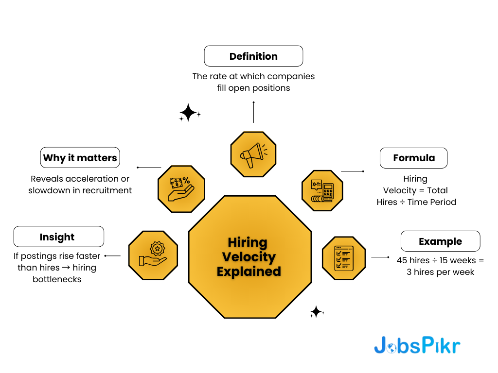
Hiring velocity measures the rate at which companies fill open positions. The formula is straightforward:

Hiring Velocity = Total Hires ÷ Time Period

For instance, if a company makes 45 hires over 15 weeks, their hiring velocity would be 3.0 hires per week. Metrics such as this will help spot acceleration or deceleration in recruitment efforts. You can also calculate hiring velocity with postings data by tracking the ratio of new postings to the filled positions. When the postings volume increases faster than hiring velocity, it signals potential hiring bottlenecks.

Adding Time-Series Smoothing

Weekly data comes with noise that hides the real trends. Moving averages help you smooth out those fluctuations and see what’s actually happening.

# Add 4-week and 8-week moving averages

weekly_data[‘ma_4w’] = weekly_data[‘postings_volume’].rolling(4).mean()

weekly_data[‘ma_8w’] = weekly_data[‘postings_volume’].rolling(8).mean()

# Calculate 95% confidence intervals

std_4w = weekly_data[‘postings_volume’].rolling(4).std()

weekly_data[‘ci_upper’] = weekly_data[‘ma_4w’] + (1.96 * std_4w)

weekly_data[‘ci_lower’] = weekly_data[‘ma_4w’] – (1.96 * std_4w)

Detecting Seasonality Patterns

Seasonality detection in time series data reveals recurring patterns that affect hiring cycles. Use statsmodels for seasonal decomposition:

from statsmodels.tsa.seasonal import seasonal_decompose

# Decompose time series into trend, seasonal, and residual components

decomposition = seasonal_decompose(weekly_data[‘postings_volume’], 

                                   model=’additive’, period=52)

You’ll notice seasonal patterns everywhere: January brings hiring surges, December slows things down, and retail spikes hard before holiday seasons.

Creating Visualization Charts

Build line charts with confidence bands to visualize hiring velocity trends:

import matplotlib.pyplot as plt

fig, ax = plt.subplots(figsize=(12, 6))

ax.plot(weekly_data.index, weekly_data[‘postings_volume’], 

        alpha=0.3, label=’Raw Data’)

ax.plot(weekly_data.index, weekly_data[‘ma_4w’], 

        linewidth=2, label=’4-Week MA’)

ax.fill_between(weekly_data.index, 

                weekly_data[‘ci_lower’], weekly_data[‘ci_upper’], 

                alpha=0.2, label=’95% CI’)

Interpreting Results

Effectiveness with trend analysis lies in separating genuine trends from seasonal noise. A spike in postings during January might reflect normal seasonal hiring rather than market growth.

Look for these patterns in your charts:

• Sustained upward trends indicate market expansion
• Seasonal spikes that return to baseline suggest normal cycles
• Volatile periods may signal economic uncertainty

Advanced Analysis Techniques

For deeper insights, compare seasonally adjusted series against raw data. This helps identify when apparent growth is actually just seasonal variation. Time series forecasting methods can extend your analysis to predict future hiring patterns based on historical trends and seasonal components. Track multiple metrics simultaneously – postings volume, hiring velocity, and time-to-fill ratios paint a complete picture of labor market dynamics.

Step 4: Forecast Demand and Turn Insights into Actions

Once you’ve collected and analyzed your job market data, the next step is building forecasts that drive real business decisions. This phase transforms raw trends into actionable workforce strategies.

Classical Forecasting Methods

Start with proven time series forecasting methods like exponential smoothing and ARIMA models. These approaches handle the natural ups and downs in hiring demand effectively. SARIMA models work particularly well for job market data because they account for seasonality. Most industries follow predictable seasonal patterns including retail hiring ramps up before holidays, education peaks during summer months. Before you build your model, run stationarity tests like ADF to make sure your data behaves predictably. Compare different model configurations using AIC scores to find the best fit for your data.

Machine Learning Enhancements

You can boost classical models by adding machine learning features. Random forest and XGBoost work well when you include lagged job postings, velocity metrics, and macro-economic indicators. These hybrid approaches capture complex relationships that pure statistical models might miss. However, keep interpretability in mind since HR stakeholders need to understand the predictions.

Building Short-Term Forecasts

Keep your forecasts to 8-12 week horizons for the best accuracy. Push beyond that and market volatility makes your predictions unreliable. Python’s statsmodels library handles SARIMA grid searches efficiently, saving you time on the technical setup. Always include prediction intervals to communicate uncertainty levels to decision makers.

Validation and Performance

Backtest your models using rolling origin validation. This method simulates real-world conditions by training on historical data and testing on future periods. Track performance using MAPE and sMAPE metrics. These measures help you understand forecast accuracy across different demand levels and time periods.

Metric	Good Performance	Needs Improvement
MAPE	< 15%	> 25%
sMAPE	< 12%	> 20%

Turning Forecasts into Action

Transform predictions into concrete workforce plans:

• Capacity Planning: Deploy recruiters based on predicted demand by role and location 
• Budget Allocation: Move spending toward high-velocity channels when demand accelerates
• Competitive Intelligence: Track how competitor companies adjust their hiring patterns

Implementation Playbook

Create automated alerts when forecasts show significant demand changes. Set up dashboards that translate predictions into recruiter workload estimates and budget recommendations. Track your competitors’ normalized posting trajectories to identify market opportunities. When their hiring slows down, you might find talent acquisition advantages.

Monitoring and Maintenance

Your models will drift as market conditions shift. Monthly monitoring helps you catch performance drops before they become problems. Plan to retrain your forecasting models every quarter or when accuracy falls below your thresholds. Keep the retraining process straightforward and well-documented for consistent results. Focus on stability over complexity when presenting to HR stakeholders. They need reliable predictions they can trust for planning purposes.

Job Market Trend Analysis: Smarter Decisions, Faster Insights

Trend analysis transforms raw labor market data into actionable workforce intelligence. You collect job postings systematically. You clean and normalize the data for accuracy. You apply statistical methods to identify patterns. You visualize trends through charts and dashboards. You interpret findings to guide strategic decisions. The timing for job market analytics has never been better. Data science roles continue showing robust growth across industries. Python adoption among practitioners creates standardized skill benchmarks for tracking. 

Real-time data gives you competitive advantages traditional reports cannot match. While quarterly surveys become outdated quickly, job data API solutions provide current market snapshots. You spot emerging skills before competitors recognize the shift. The combination of data freshness, normalization accuracy, and broad coverage accelerates your time-to-insight. You build confident forecasts based on current market conditions rather than historical assumptions. Global hiring patterns in 2025 demonstrate how quickly labor markets evolve. Organizations using real-time trend analysis adapt faster to changing workforce demands.

FAQs